
| 일 | 월 | 화 | 수 | 목 | 금 | 토 |
|---|---|---|---|---|---|---|
| 1 | 2 | 3 | 4 | 5 | 6 | |
| 7 | 8 | 9 | 10 | 11 | 12 | 13 |
| 14 | 15 | 16 | 17 | 18 | 19 | 20 |
| 21 | 22 | 23 | 24 | 25 | 26 | 27 |
| 28 | 29 | 30 | 31 |
- 딥러닝
- c언어
- 파이토치 김성훈 교수님 강의 정리
- 딥러닝 공부
- pytorch
- 모두의 딥러닝
- 영상처리
- MFC 프로그래밍
- tensorflow 예제
- c++
- 팀프로젝트
- 파이토치 강의 정리
- TensorFlow
- C언어 공부
- 파이토치
- pytorch zero to all
- matlab 영상처리
- object detection
- 컴퓨터 비전
- c언어 정리
- 가우시안 필터링
- 케라스 정리
- 미디언 필터링
- 딥러닝 스터디
- c++공부
- 해리스 코너 검출
- 골빈해커
- Pytorch Lecture
- 모두의 딥러닝 예제
- 김성훈 교수님 PyTorch
- Today
- Total
ComputerVision Jack
[모두의 딥러닝 Chapter11] 본문
[11-0 cnn_basics]
합성곱 신경망에 대한 기본
sess = tf.InteractiveSession()
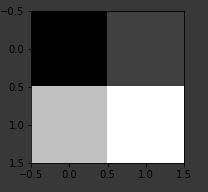
image = np.array([[[[1],[2],[3]],
[[4],[5],[6]],
[[7],[8],[9]]]], dtype=np.float32)
print(image.shape)
plt.imshow(image.reshape(3,3), cmap='Greys')
#기본적인 예제 이미지 생성

print("image.shape", image.shape)
weight = tf.constant([[[[1.]],[[1.]]],
[[[1.]],[[1.]]]])
print("weight.shape", weight.shape)
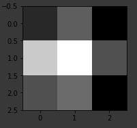
conv2d = tf.nn.conv2d(image, weight, strides=[1, 1, 1, 1], padding='VALID')
conv2d_img = conv2d.eval()
print("conv2d_img.shape", conv2d_img.shape)
conv2d_img = np.swapaxes(conv2d_img, 0, 3)
for i, one_img in enumerate(conv2d_img):
print(one_img.reshape(2,2))
plt.subplot(1,2,i+1), plt.imshow(one_img.reshape(2,2), cmap='gray')
#tf.nn.conv2d()메소드를 사용하여 원 이미지에 마스크 이미지(weight)을 연산한 결과를 출력하는 부분.
weight을 마스크 처럼 취급하여 영상에 대해 strides = [1, 1]이기 때문에 한칸씩 이동하면서 원 본 이미지에
가중치를 연산하여 결과를 출력한다.
padding = 'VALID'
패딩에 관련된 내용은 영상을 마스크 연산 적용할 떄, 외각선을 처리해주는 내용과 같다.
3 X 3 이미지에 마스크 2 X 2를 적용하면 결과적으로 2 X 2 영상이 도출되고,
우리가 입력으로 준영상이 2 X 2 로 축소된것을 확인할 수 있다.
padding = 'SAME'
conv2d = tf.nn.conv2d(image, weight, strides=[1, 1, 1, 1], padding='SAME')
conv2d_img = conv2d.eval()
인자를 SAME으로 하면 외각선이 자동으로 마스크연산 크기에 맞게 늘어난다.
따라서 3 X 3영상이 외각 부분이 한칸씩 늘어 5 X 5 영상이 된다. 여기에 2 X 2 마스크를 적용하면,
결과적으로 3 X 3영상이 도출된다.
print("image.shape", image.shape)
weight = tf.constant([[[[1.,10.,-1.]],[[1.,10.,-1.]]],
[[[1.,10.,-1.]],[[1.,10.,-1.]]]])
print("weight.shape", weight.shape)
conv2d = tf.nn.conv2d(image, weight, strides=[1, 1, 1, 1], padding='SAME')
conv2d_img = conv2d.eval()
print("conv2d_img.shape", conv2d_img.shape)
conv2d_img = np.swapaxes(conv2d_img, 0, 3)
for i, one_img in enumerate(conv2d_img):
print(one_img.reshape(3,3))
plt.subplot(1,3,i+1), plt.imshow(one_img.reshape(3,3), cmap='gray')
#다양한 weight(마스크)를 사용하여 연산한 결과를 출력해 보는 부분.

Max Pooling
영상을 가져와서 마스크 사이즈만큼 흩어 내려 갈 때, stride 크기를 고려하여 최대값을 뽑아내는것.
[[1, 2], [3, 4] 인 경우 마스크 사이즈가 [2 x 2]이고 strides크기가 [1 x 1]인경우 max pooling을 적용하면
결과로 4가 출력된다.
마찬가지로 padding에 의해 영향을 받는다.
sess = tf.InteractiveSession()
img = img.reshape(-1, 28, 28, 1)
W1 = tf.Variable(tf.random_normal([3, 3, 1, 5], stddev=0.01))
conv2d = tf.nn.conv2d(img, W1, strides = [1, 2, 2, 1], padding = 'SAME')
print(conv2d)
sess.run(tf.global_variables_initializer())
conv2d_img = conv2d.eval()
conv2d_img = np.swapaxes(conv2d_img, 0, 3)
for i, one_img in enumerate(conv2d_img):
plt.subplot(1, 5, i + 1), plt.imshow(one_img.reshape(14, 14), cmap = 'gray')
#mnist자료형을 읽어와 작업
img size = (28 x 28 레이어 1)
W경우 [3 x 3] 마스크를 사용하고 레이어 크기는 1, 결과로 뽑아낼 층 갯수 5
padding을 same으로 적용하여 stride 크기는 [2 x 2]로 conv2d()연산을 수행한다.

pool = tf.nn.max_pool(conv2d, ksize = [1, 2, 2, 1], strides = [1, 2, 2, 1], padding = 'SAME')
print(pool)
sess.run(tf.global_variables_initializer())
pool_img = pool.eval()
pool_img = np.swapaxes(pool_img, 0, 3)
for i, one_img in enumerate(pool_img):
plt.subplot(1, 5, i + 1), plt.imshow(one_img.reshape(7, 7), cmap = 'gray')
#연산된 conv2d에서 max_pooling을 적용하는 부분.

[11-1 mnist_cnn]
mnist자료에 대해 cnn을 적용하여 모델 구현
learning_rate = 0.001
training_epochs = 15
batch_size = 100
#하이퍼 파라미터를 설정한다.
X = tf.placeholder(tf.float32, [None, 784])
X_img = tf.reshape(X, [-1, 28, 28, 1])
Y = tf.placeholder(tf.float32, [None, 10])
#X데이터 같은 경우 이번엔 영상 전체를 통으로 입력하지 않기 때문에 [784] - [28, 28]로 reshape을 적용한다.
W1 = tf.Variable(tf.random_normal([3, 3, 1, 32], stddev = 0.01))
L1 = tf.nn.conv2d(X_img, W1, strides = [1, 1, 1, 1], padding = 'SAME')
L1 = tf.nn.relu(L1)
L1 = tf.nn.max_pool(L1, ksize = [1, 2, 2, 1],
strides = [1, 2, 2, 1], padding = 'SAME')
#첫번째 층에서 [3 x 3] 마스크를 이용해 32개의 층을 뽑아낸다.
relu활성 함수를 적용하고, max_pooling을 적용해 [28 * 28] 영상이 [14 * 14]로 반토막난다. stride가 [2, 2]이기 때문에.
W2 = tf.Variable(tf.random_normal([3, 3, 32, 64], stddev = 0.01))
L2 = tf.nn.conv2d(L1, W2, strides = [1, 1, 1, 1], padding = 'SAME')
L2 = tf.nn.relu(L2)
L2 = tf.nn.max_pool(L2, ksize = [1, 2, 2, 1],
strides = [1, 2, 2, 1], padding = 'SAME')
#다음 층은 첫번째 32개의 층을 가져와 64개의 층으로 내보낸다.
relu활성함수를 넣고, 마찬가지로 max_pooling을 적용하면 [7 * 7]사이즈의 이미지가 출력이 된다.
L2_flat = tf.reshape(L2, [-1, 7 * 7 * 64])
#다음 출력 [7 * 7] 이미지 64개를 flatten하여 옆으로 길게 나열한다.
W3 = tf.get_variable("W3", shape= [7 * 7 * 64, 10],
initializer = tf.contrib.layers.xavier_initializer())
b = tf.Variable(tf.random_normal([10]))
logits = tf.matmul(L2_flat, W3) + b
#softmax함수를 적용하여, 분류를 실행한다.
분류를 실행하기 위해 마지막으로 나온 결과를 flatten한다고 생각해도 된다.
전의 mnist데이터 학습처럼 진행해 나아가면 된다.
[11-2 mnist_deep_cnn]
합성곱 신경망을 깊게 생성하기
W3 = tf.Variable(tf.random_normal([3, 3, 64, 128], stddev = 0.01))
L3 = tf.nn.conv2d(L2, W3, strides = [1, 1, 1, 1], padding = 'SAME')
L3 = tf.nn.relu(L3)
L3 = tf.nn.max_pool(L3, ksize = [1, 2, 2, 1], strides = [1, 2, 2, 1], padding= 'SAME')
L3 = tf.nn.dropout(L3, keep_prob = keep_prob)
#전 예제의 L2에 L3을 연결하기만 하면된다. 64개층의 을 입력으로 사용하여 128개의 층을 뽑아낸다.
전 층에서 [7 * 7]영상이 나왔기 때문에 맥스 풀링을 적용하면, [4 * 4] 이미지가 나온다.
W3 = tf.Variable(tf.random_normal([3, 3, 64, 128], stddev = 0.01))
L3 = tf.nn.conv2d(L2, W3, strides = [1, 1, 1, 1], padding = 'SAME')
L3 = tf.nn.relu(L3)
L3 = tf.nn.max_pool(L3, ksize = [1, 2, 2, 1], strides = [1, 2, 2, 1], padding= 'SAME')
L3 = tf.nn.dropout(L3, keep_prob = keep_prob)
# 기존 softmax실습을 했던것 처럼 신경망을 쌓아간다.(그러기 위한 flatten)
W5 = tf.get_variable("W5", shape=[625, 10],
initializer=tf.contrib.layers.xavier_initializer())
b5 = tf.Variable(tf.random_normal([10]))
logits = tf.matmul(L4, W5) + b5
#결과가 10개로 분류되기 떄문에 마지막은 결국 10이다.
[11-3 mnist_cnn_class]
파이썬도 객체 지향 프로그래밍 언어이다. 따라서 우리가 자주 사용했던 클래스로 모듈화를 진행 할 수 있다.
클래스 모듈화
class Model:
def __init__(self, sess, name):
self.sess = sess
self.name = name
self._build_net()
def _build_net(self):
with tf.variable_scope(self.name):
self.keep_prob = tf.placeholder(tf.float32)
self.X = tf.placeholder(tf.float32, [None, 784])
X_img = tf.reshape(self.X, [-1, 28, 28, 1])
self.Y = tf.placeholder(tf.float32, [None, 10])
W1 = tf.Variable(tf.random_normal([3, 3, 1, 32], stddev=0.01))
L1 = tf.nn.conv2d(X_img, W1, strides=[1, 1, 1, 1], padding='SAME')
L1 = tf.nn.relu(L1)
L1 = tf.nn.max_pool(L1, ksize=[1, 2, 2, 1],
strides=[1, 2, 2, 1], padding='SAME')
L1 = tf.nn.dropout(L1, keep_prob=self.keep_prob)
W2 = tf.Variable(tf.random_normal([3, 3, 32, 64], stddev=0.01))
L2 = tf.nn.conv2d(L1, W2, strides=[1, 1, 1, 1], padding='SAME')
L2 = tf.nn.relu(L2)
L2 = tf.nn.max_pool(L2, ksize=[1, 2, 2, 1],
strides=[1, 2, 2, 1], padding='SAME')
L2 = tf.nn.dropout(L2, keep_prob=self.keep_prob)
W3 = tf.Variable(tf.random_normal([3, 3, 64, 128], stddev=0.01))
L3 = tf.nn.conv2d(L2, W3, strides=[1, 1, 1, 1], padding='SAME')
L3 = tf.nn.relu(L3)
L3 = tf.nn.max_pool(L3, ksize=[1, 2, 2, 1], strides=[
1, 2, 2, 1], padding='SAME')
L3 = tf.nn.dropout(L3, keep_prob=self.keep_prob)
L3_flat = tf.reshape(L3, [-1, 128 * 4 * 4])
W4 = tf.get_variable("W4", shape=[128 * 4 * 4, 625],
initializer=tf.contrib.layers.xavier_initializer())
b4 = tf.Variable(tf.random_normal([625]))
L4 = tf.nn.relu(tf.matmul(L3_flat, W4) + b4)
L4 = tf.nn.dropout(L4, keep_prob=self.keep_prob)
W5 = tf.get_variable("W5", shape=[625, 10],
initializer=tf.contrib.layers.xavier_initializer())
b5 = tf.Variable(tf.random_normal([10]))
self.logits = tf.matmul(L4, W5) + b5
self.cost = tf.reduce_mean(tf.nn.softmax_cross_entropy_with_logits_v2(
logits=self.logits, labels=self.Y))
self.optimizer = tf.train.AdamOptimizer(
learning_rate=learning_rate).minimize(self.cost)
correct_prediction = tf.equal(
tf.argmax(self.logits, 1), tf.argmax(self.Y, 1))
self.accuracy = tf.reduce_mean(tf.cast(correct_prediction, tf.float32))
def predict(self, x_test, keep_prop=1.0):
return self.sess.run(self.logits, feed_dict={self.X: x_test, self.keep_prob: keep_prop})
def get_accuracy(self, x_test, y_test, keep_prop=1.0):
return self.sess.run(self.accuracy, feed_dict={self.X: x_test, self.Y: y_test, self.keep_prob: keep_prop})
def train(self, x_data, y_data, keep_prop=0.7):
return self.sess.run([self.cost, self.optimizer], feed_dict={
self.X: x_data, self.Y: y_data, self.keep_prob: keep_prop})
#기존 셀 단위로 실행했던 것을 클래스로 묶어서 사용한다.
[11-4 mnist_cnn_layers]
conv1 = tf.layers.conv2d(inputs=X_img, filters=32, kernel_size=[3, 3],
padding="SAME", activation=tf.nn.relu)
pool1 = tf.layers.max_pooling2d(inputs=conv1, pool_size=[2, 2],
padding="SAME", strides=2)
dropout1 = tf.layers.dropout(inputs=pool1,rate=0.3, training=self.training)
#API를 사용하여 layers를 사용하여 제작한다.
[11-5] mnist_cnn_ensemble_layers]
sess = tf.Session()
models = []
num_models = 2
for m in range(num_models):
models.append(Model(sess, "model" + str(m)))
sess.run(tf.global_variables_initializer())
print('Learning Started!')
#모델을 여러개 생성하여 모델별로 학습한 결과를 ensemble하여 결과를 제시한다.
하나의 모델을 사용했을 때보다 일반화에 대해 좀더 이점이 있다.
test_size = len(mnist.test.labels)
predictions = np.zeros([test_size, 10])
for m_idx, m in enumerate(models):
print(m_idx, 'Accuracy:', m.get_accuracy(
mnist.test.images, mnist.test.labels))
p = m.predict(mnist.test.images)
predictions += p
ensemble_correct_prediction = tf.equal(
tf.argmax(predictions, 1), tf.argmax(mnist.test.labels, 1))
ensemble_accuracy = tf.reduce_mean(
tf.cast(ensemble_correct_prediction, tf.float32))
print('Ensemble accuracy:', sess.run(ensemble_accuracy))
#앙상블 결과 확인 부분.
[11-X mnist_cnn_low_memory]
다음 부수적 예제는 cnn에 들어갈 mnist데이터가 메모리 적으로 효율을 보게 작성된 코드이다.
'DeepLearning > DL_ZeroToAll' 카테고리의 다른 글
| [모두의 딥러닝 Chapter12] (0) | 2020.01.28 |
|---|---|
| [모두의 딥러닝 Chapter10] (0) | 2020.01.22 |
| [모두의 딥러닝 Chapter09] (0) | 2020.01.21 |
| [모두의 딥러닝 Chapter08] (0) | 2020.01.20 |
| [모두의 딥러닝 Chapter07] (0) | 2020.01.19 |

