
| 일 | 월 | 화 | 수 | 목 | 금 | 토 |
|---|---|---|---|---|---|---|
| 1 | ||||||
| 2 | 3 | 4 | 5 | 6 | 7 | 8 |
| 9 | 10 | 11 | 12 | 13 | 14 | 15 |
| 16 | 17 | 18 | 19 | 20 | 21 | 22 |
| 23 | 24 | 25 | 26 | 27 | 28 | 29 |
| 30 |
- pytorch
- 영상처리
- tensorflow 예제
- object detection
- 미디언 필터링
- 해리스 코너 검출
- C언어 공부
- 김성훈 교수님 PyTorch
- pytorch zero to all
- c언어 정리
- 파이토치 김성훈 교수님 강의 정리
- 모두의 딥러닝 예제
- 케라스 정리
- 파이토치
- 딥러닝
- c언어
- c++
- 딥러닝 공부
- c++공부
- 가우시안 필터링
- 골빈해커
- 파이토치 강의 정리
- 팀프로젝트
- Pytorch Lecture
- matlab 영상처리
- TensorFlow
- 딥러닝 스터디
- 컴퓨터 비전
- 모두의 딥러닝
- MFC 프로그래밍
- Today
- Total
ComputerVision Jack
PyTorch Lecture 09 : softmax Classifier 본문
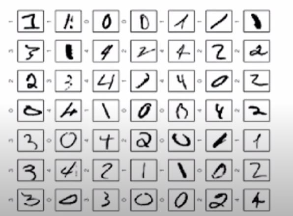
MNIST input
이번 시간엔 MNIST (숫자 그림 자료)데이터로 각각 해당 숫자에 맞게 분류하는 시간이었습니다.
MNIST 데이터는 딥러닝을 공부할 때 기본이 되는 데이터로, 가로 28p 세로 28p 컬러값 1인 숫자 이미지 파일입니다.
지난 시간 저희는 간단하게 다변수에 대한 이진 결과를 예측하는 모델(logistic regression)을 만들었습니다.
이번엔 다변수에 대한 결과를 각각해당 class에 맞게 분류하는 모델을 만들려고합니다.
10 outputs
예전 모델을 생각해본다면 X -> Linear -> Activation Function -> Y_pred 입니다.
따라서 선형 모델에서 x_data의 shape이 (n, 2) 이라면 w의 shape은 (2, 1)되어 y의 shape은 자동으로 (n, 1)이 됩니다.
결과를 10개의 클래스로 구분해야 한다면, x shape(n, 784) w (? , ?) y shape(n, 10)이면 w shape의 유추가 가능하신가요? 네 행렬곱의 연산을 떠올리시면 w는 (784, 10)으로 shape을 떠올릴 수 있습니다.
또한 결과가 여러개의 클래스로 분류되는 모델은 X -> Linear -> Softmax - > Y_pred( 0.7, 0.2, 0.1) 이런식으로 나오게됩니다.
softmax 함수
softmax 함수는 해당 변수의 값을 0 ~ 1 사이의 값으로 변경합니다. 수식은 -Y * logY^ 입니다.
따라서 MNIST의 데이터를 적용해 본다면, [ 0.7, 0.3, 0.4, 0.5,,,,10개] 로 0~9까지의 결과값이 표기됩니다.
one-hot 코딩
one-hot 코딩은 해당 softmax로 출력된 값에 대해 가장 높은 값을 1로 취하고 나머지를 0으로 만들어 분류값의 편의를 봐주는 코딩방식입니다. 따라서 4에 해당하는 값은 [0, 0, 0, 0, 1, 0, 0, 0, 0, 0] 가 됩니다.
[09.1_softmax_loss.py]
해당 예제는 softmax의 값의 손실함수적 측면을 알아보는 코드입니다.
코렙으로 코드를 구현할 때 주의할 점은 'numpy.ndarray' object has no attribute 'log_softmax'
오류를 마주할 수 있습니다. 이경우 numpy의 버전 오류이기 때문에 코드를 돌리기 전에
!pip install numpy==1.3.0 을 적용하여 numpy 버전을 다운그레이드 해주시면 됩니다.
[09.2_softmax_mnist.py]
이제 실질적은 mnist 데이터셋의 분류를 softmax 함수를 이용하여 구현해보겠습니다.
from __future__ import print_function
from torch import nn, optim, cuda
from torch.utils import data
from torchvision import datasets, transforms
import torch.nn.functional as F
import time
# 해당 프로젝트 구현에 필요한 라이브러리를 import 합니다.
batch_size = 64
device = 'cuda' if cuda.is_available() else 'cpu'
print(f'Training MNIST Model on {device}\n{"=" * 44}')
# 해당 MNIST의 batch_size를 64로 설정하고 cuda 환경 체크하기 위한 코드를 진행합니다. 해당 프로젝트 경우 데이터 셋도 작고 cpu로 충분히 돌릴 수 있기 때문에 그냥 진행하셔도 됩니다.
train_dataset = datasets.MNIST(root='./mnist_data', train = True, transform = transforms.ToTensor(), download=True)
test_dataset = datasets.MNIST(root='./mnist_data/', train = False, transform = transforms.ToTensor())
#MNIST 데이터 셋을 다운받습니다. train_dataset 경우 학습을 진행하기 위해 필요한 데이터셋이며 test 데이터셋 경우
해당 학습한 모델의 정확도를 파악하기 위해 사용합니다.
train_loader = data.DataLoader(dataset = train_dataset, batch_size = batch_size, shuffle=True)
test_loader = data.DataLoader(dataset = test_dataset, batch_size = batch_size, shuffle = False)
# 다운 받은 각각의 dataset에 대해 DataLoader를 제작합니다.
class Net(nn.Module):
def __init__(self):
super(Net, self).__init__()
self.l1 = nn.Linear(784, 520)
self.l2 = nn.Linear(520, 320)
self.l3 = nn.Linear(320, 240)
self.l4 = nn.Linear(240, 120)
self.l5 = nn.Linear(120, 10)
def forward(self, x):
x = x.view(-1, 784) # Flatten the data(n, 1, 28, 28) - > (n, 784)
x = F.relu(self.l1(x))
x = F.relu(self.l2(x))
x = F.relu(self.l3(x))
x = F.relu(self.l4(x))
return self.l5(x)
# 이제 네트워크를 구성합니다. mnist의 데이터 셋은 (28 * 28(면적)) 이기 때문에 784의 특징이되고, 출력은 0~9까지 10개의 분류를 진행하기 때문에 초기엔 784로 특직을 받고 출력에선 10으로 끝나야합니다.
또한 forward 함수 부분에서 view 함수를 통해 데이터 플래튼(reshape)을 진행했습니다. 원래 mnist 데이터셋은 2차원인 행렬 데이터 셋입니다. 하지만 1차원으로 차원을 축소하여 (28 ,28) -> (1, 784)로 바꿨다고 할 수 있습니다.
model = Net()
model.to(device)
# 해당 모델의 객체를 생성합니다.
criterion = nn.CrossEntropyLoss()
optimizer = optim.SGD(model.parameters(), lr = 0.01, momentum = 0.5)
# 생성한 모델의 손실함수(crossEntropy)를 생성하고 최적화 부분을 진행합니다.
def train(epoch):
model.train()
for batch_idx, (data, target) in enumerate(train_loader):
data, target = data.to(device), target.to(device)
optimizer.zero_grad()
output = model(data)
loss = criterion(output, target)
loss.backward()
optimizer.step()
if batch_idx % 10 == 0:
print('Train Epoch : {} | Batch Status : {} / {} ({:.0f}%) | Loss : {:.6f}'.format(
epoch, batch_idx * len(data), len(train_loader.dataset), 100. * batch_idx / len(train_loader), loss.item()
))
# train Loader에 들어있는 학습에 필요한 데이터를 읽어와 학습을 진행합니다.
def test():
model.eval()
test_loss = 0
correct = 0
for data, target in test_loader:
data, target = data.to(device), target.to(device)
output = model(data)
# sum up batch loss
test_loss += criterion(output, target).item()
# get the index of the max
pred = output.data.max(1, keepdim=True)[1]
correct += pred.eq(target.data.view_as(pred)).cpu().sum()
test_loss /= len(test_loader.dataset)
print(f'===========================\nTest set: Average loss: {test_loss:.4f}, Accuracy: {correct}/{len(test_loader.dataset)} '
f'({100. * correct / len(test_loader.dataset):.0f}%)')
# 학습된 모델에 대해 test_loader에서 데이터를 꺼내와 결과를 예측합니다. 결과에 대한 값을 통계 내어 정확도로 사용합니다.
if __name__ == '__main__':
since = time.time()
for epoch in range(1, 10):
epoch_start = time.time()
train(epoch)
m, s = divmod(time.time() - epoch_start, 60)
print(f'Training time: {m:.0f}m {s:.0f}s')
test()
m, s = divmod(time.time() - epoch_start, 60)
print(f'Testing time: {m:.0f}m {s:.0f}s')
m, s = divmod(time.time() - since, 60)
print(f'Total Time: {m:.0f}m {s:.0f}s\nModel was trained on {device}!')
# 총 해당 batch_size로 나눈 데이터에 대해 10번의 epoch으로 반복을 진행합니다. 따라서 전체 데이터를 10번 반복하며 학습을 진행합니다. 그다음 한번의 epoch의 진행되면 test case를 실험하여 정확도를 추출합니다. epoch이 늘어날 수록 test case에 대한 정확도도 올라가는 것을 확인 할 수 있습니다.
'DeepLearning > Pytorch_ZeroToAll' 카테고리의 다른 글
| PyTorch Lecture 11 : Advanced CNN (0) | 2020.10.27 |
|---|---|
| PyTorch Lecture 10 : Basic CNN (0) | 2020.10.26 |
| PyTorch Lecture 08 : DataLoader (0) | 2020.10.21 |
| PyTorch Lecture 07 : Wide and Deep (0) | 2020.10.20 |
| PyTorch Lecture 06 : Logistic Regression (0) | 2020.10.12 |


